Electricity Power Plants in the United States
This project will explore the electricity generation plants in the United States and their air pollutants and greenhouse gas (GHG) emissions. There are three parts in this porject.
Part one explores the average electricity GHG emission factor on a state level and how they are affected by the electricty mix in different state (renewable-to-total and natural-gas-to-fossil-fuel). In carbon accounting, this is called scope II emission.
Part two explores the generation plants in ten most populated states, and their total \(NO_x\), \(SO_2\), and GHG emission in 2018.
Part three explores the electricity generation and emissions for California counties in 2018.
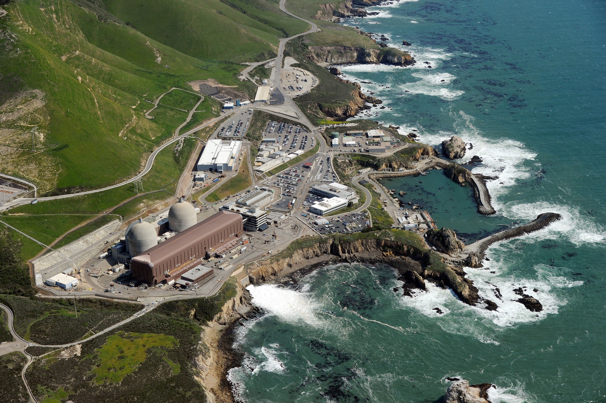
Figure 1. The Diablo Canyon Nuclear Power Plant. Located in San Luis Obispo county, the Diablo Canyon nuclear power plant is the last operating nuclear power plant in California. (Source: The New York Times, 2016)
#Read in data sets.

raw_df <- read_excel("egrid2018_data.xlsx", skip = 1, sheet = "PLNT18")
raw_df_st <- read_excel("egrid2018_data.xlsx", skip = 1, sheet = "ST18")
clean_df <- raw_df %>%
clean_names() %>%
select(pstatabb, cntyname, fipsst, fipscnty, plprmfl, plfuelct, coalflag, namepcap, plnoxrta, plso2rta, plco2rta, plch4rta, pln2orta, plc2erta, plso2an, plnoxan, plco2eqa, plngenan) #Selecting the cateogries of interestclean_st_df <- raw_df_st %>%
clean_names() %>%
select(pstatabb, stnoxrta, stso2rta, namepcap, stgenatn, stc2erta, sttrpr, stgspr, sttnpr, stngenan) %>%
mutate(gas_ratio = stgspr/sttnpr) #Calculating the percentage of gas-generated electricity among all fossil fuel-generated electricity.Part One. The average electricity GHG emission factor on a state level.
state_bubble <- ggplot(clean_st_df, aes(x = sttrpr*100, y = stc2erta, size = stngenan)) +
  geom_point(alpha = 0.8, color = "#5BBCD6")+
  scale_size(range = c(.1, 10), name="Total Generation (MWh)")+
  xlab("Renewable Electricity Percentage")+
  ylab("Average Electricity GHG Emission Factor (lb/MWh)")+
  geom_text_repel(aes(label = pstatabb), size = 2)+
  theme_classic()


state_bubble
Figure 2. The Relationship between Average Electricity GHG Emission Factor and Renewable Generation Percentage on a State Level. Each bubble stands for a state. The size of the bubble indicates the total electricity generation in the state. The data for generation and GHG emission are from the year of 2018. (Source: eGrid, 2018)
clean_st_fossil <- clean_st_df %>%
  filter(sttnpr > 0.80)

state_fs_bubble <- ggplot(clean_st_fossil, aes(x = gas_ratio*100, y = stc2erta, size = stngenan)) +
  geom_point(alpha = 0.8, color = "#F98400")+
  scale_size(range = c(.1, 10), name="Total Generation (MWh)")+
  xlab("Pencentage of Natural-gas-electricity among Fossil-fuel-electricity")+
  ylab("Average Electricity GHG Emission Factor (lb/MWh)")+
  geom_text_repel(aes(label = pstatabb), size = 2)+
  theme_classic()

state_fs_bubble
Figure 3. The Relationship between Average Electricity GHG Emission Factor and the Pencentage of Natural-gas-electricity among Fossil-fuel-electricity for States with More than 80% Non-renewable Electricity. Each bubble stands for a state. The size of the bubble indicates the total electricity generation in the state. The data for generation and GHG emission are from the year of 2018. (Source: eGrid, 2018)
Part Two. The generation plants in ten most populated states.
gas_df <- clean_df %>%
  filter (plfuelct %in% c("GAS", "OIL", "COAL"))%>% # Selecting all fossil fuels
  group_by(pstatabb) %>%
  select(-coalflag) %>%
  drop_na() %>%
  filter(pstatabb %in% c("CA", "TX", "FL", "NY", "PA", "IL", "OH", "GA", "NC", "MI"))# Selecting the top ten populated states
gasvis2 <- ggplot(gas_df, aes(x = pstatabb, y = plso2an))+
geom_jitter(width = 0.20, aes(color = plfuelct))+
theme_classic()+
scale_y_continuous(expand = c(0, 0))+
scale_color_manual(values=wes_palette(n=3, name="Darjeeling1"))+
xlab("State")+
ylab("2018 Annual Sulfur Dioxide Emssion (tons)")+
labs(color = "Plant Type")
gasvis2
Figure 4. Total Annual \(SO_2\) Emission on a Power Plant Level for Ten Most Populated States. Each point stands for a power plant. The color of the point indicates the type of the power plant. The data for generation and GHG emission are from the year of 2018. (Source: eGrid, 2018)
gasvis4 <- ggplot(gas_df, aes(x = pstatabb))+
  geom_jitter(width = 0.20, aes(y = plnoxan,color = plfuelct))+
  theme_classic()+
  scale_y_continuous(expand = c(0, 0))+
  scale_color_manual(values=wes_palette(n=3, name="Darjeeling1"))+
  xlab("State")+
  ylab("2018 Annual NOx Emssion (tons)")+
  labs(color = "Plant Type")

gasvis4
Figure 5. Total Annual \(NO_x\) Emission on a Power Plant Level for Ten Most Populated States. Each point stands for a power plant. The color of the point indicates the type of the power plant. The data for generation and GHG emission are from the year of 2018. (Source: eGrid, 2018)
gasvis5 <- ggplot(gas_df, aes(x = pstatabb))+
  geom_jitter(width = 0.20, aes(y = plco2eqa,color = plfuelct))+
  theme_classic()+
  scale_y_continuous(expand = c(0, 0))+
  scale_color_manual(values=wes_palette(n=3, name="Darjeeling1"))+
  xlab("State")+
  ylab("2018 Annual GHG Emssion (tons carbon dioxide equivalent)")+
  labs(color = "Plant Type")

gasvis5
Figure 6. Total Annual GHG Emission on a Power Plant Level for Ten Most Populated States. Each point stands for a power plant. The color of the point indicates the type of the power plant. The data for generation and GHG emission are from the year of 2018. (Source: eGrid, 2018)
Part Three. Electricity generation and emissions for California counties
ca_df <- clean_df %>%
  filter(pstatabb == "CA") %>%
  select(-coalflag) %>%
  mutate(cntyname = str_to_title(cntyname)) %>%
  group_by(cntyname) %>%
  mutate(plso2an = replace_na(plso2an, 0)) %>%
  mutate(plnoxan = replace_na(plnoxan, 0)) %>%
  filter (is.na (plngenan) == FALSE) %>%
  summarise(nox_total = sum(plnoxan),
            so2_total = sum(plso2an),
            gen_total = sum(plngenan)) %>%
  mutate(nox_rt = scales::number(nox_total*2000/gen_total, accuracy = 0.001),
         so2_rt = scales::number(so2_total*2000/gen_total, accuracy = 0.001)) %>%
  mutate(nox_rt = cell_spec(nox_rt, "html", bold = T, color = ifelse(nox_rt > 0.377, "#F2AD00", "#00A08A"), background = "#d7eff5"),
         so2_rt = cell_spec(so2_rt, "html", bold = T, color = ifelse(so2_rt > 0.036, "#F2AD00", "#00A08A"), background = "#d7eff5"))


title <- c("County", "Total NOx Emission (tons)", "Total SO2 Emission (tons)", "Total Net Generation (MWh)", "NOx Emission Rate (lb/MWh)", "SO2 Emission Rate(lb/MWh)")

colnames(ca_df) <- title
my_tbl <- ca_df %>%
kable(escape=F, align = "r") %>%
kable_styling(bootstrap_options = c("striped", "hover", "condensed")) %>%
column_spec(1, bold = T, color = "white", background = "#046C9A") %>%
row_spec(0, bold = T, color = "white", background = "#F98400")%>%
scroll_box(width = "100%", height = "300px")| County | Total NOx Emission (tons) | Total SO2 Emission (tons) | Total Net Generation (MWh) | NOx Emission Rate (lb/MWh) | SO2 Emission Rate(lb/MWh) |
|---|---|---|---|---|---|
| Alameda | 723.060 | 23.439 | 2033905.00 | 0.711 | 0.023 |
| Amador | 0.000 | 0.000 | 738753.00 | 0.000 | 0.000 |
| Butte | 8.811 | 2.135 | 2353681.00 | 0.007 | 0.002 |
| Calaveras | 0.000 | 0.000 | 493930.00 | 0.000 | 0.000 |
| Colusa | 163.039 | 34.964 | 3152517.00 | 0.103 | 0.022 |
| Contra Costa | 3419.368 | 58.228 | 14286071.00 | 0.479 | 0.008 |
| El Dorado | 167.884 | 0.200 | 1360204.00 | 0.247 | 0.000 |
| Fresno | 256.030 | 39.102 | 6871723.00 | 0.075 | 0.011 |
| Glenn | 0.000 | 0.000 | 7791.00 | 0.000 | 0.000 |
| Humboldt | 4732.149 | 49.976 | 536932.00 | 17.627 | 0.186 |
| Imperial | 54.158 | 1413.840 | 8388389.07 | 0.013 | 0.337 |
| Inyo | 0.000 | 549.855 | 1373519.00 | 0.000 | 0.801 |
| Kern | 6663.567 | 122.718 | 32066102.00 | 0.416 | 0.008 |
| Kings | 268.177 | 0.526 | 1197595.00 | 0.448 | 0.001 |
| Lake | 1.306 | 0.270 | 943400.00 | 0.003 | 0.001 |
| Lassen | 423.338 | 33.600 | 274015.00 | 3.090 | 0.245 |
| Los Angeles | 8013.808 | 497.241 | 22910992.61 | 0.700 | 0.043 |
| Madera | 283.825 | 0.490 | 890244.99 | 0.638 | 0.001 |
| Marin | 0.000 | 5.402 | 29920.00 | 0.000 | 0.361 |
| Mariposa | 0.000 | 0.000 | 269655.00 | 0.000 | 0.000 |
| Mendocino | 0.000 | 0.000 | 19041.00 | 0.000 | 0.000 |
| Merced | 28.840 | 0.158 | 251373.00 | 0.229 | 0.001 |
| Mono | 0.000 | 0.000 | 400981.00 | 0.000 | 0.000 |
| Monterey | 257.263 | 16.413 | 4975840.84 | 0.103 | 0.007 |
| Napa | 0.000 | 0.000 | 1566.00 | 0.000 | 0.000 |
| Nevada | 0.000 | 0.000 | 273679.00 | 0.000 | 0.000 |
| Orange | 1995.386 | 81.375 | 1442024.21 | 2.767 | 0.113 |
| Placer | 181.772 | 46.269 | 1976944.00 | 0.184 | 0.047 |
| Plumas | 120.342 | 20.313 | 1342157.00 | 0.179 | 0.030 |
| Riverside | 400.508 | 74.247 | 9105865.01 | 0.088 | 0.016 |
| Sacramento | 147.373 | 27.541 | 6315421.00 | 0.047 | 0.009 |
| San Benito | 0.000 | 0.000 | 220169.00 | 0.000 | 0.000 |
| San Bernardino | 983.456 | 17.332 | 10593186.84 | 0.186 | 0.003 |
| San Diego | 2076.426 | 45.743 | 4825121.99 | 0.861 | 0.019 |
| San Francisco | 221.592 | 0.928 | 103400.00 | 4.286 | 0.018 |
| San Joaquin | 444.818 | 18.047 | 2870108.00 | 0.310 | 0.013 |
| San Luis Obispo | 2.446 | 2.098 | 20619666.00 | 0.000 | 0.000 |
| San Mateo | 114.136 | 15.055 | 128516.00 | 1.776 | 0.234 |
| Santa Barbara | 13.808 | 4.696 | 193125.00 | 0.143 | 0.049 |
| Santa Clara | 435.387 | 10.611 | 3693010.01 | 0.236 | 0.006 |
| Santa Cruz | 29.756 | 6.015 | 60099.00 | 0.990 | 0.200 |
| Shasta | 580.339 | 106.119 | 6563004.00 | 0.177 | 0.032 |
| Sierra | 89.447 | 9.504 | 71384.00 | 2.506 | 0.266 |
| Siskiyou | 57.415 | 3.879 | 324458.00 | 0.354 | 0.024 |
| Solano | 402.206 | 16.717 | 3182720.00 | 0.253 | 0.011 |
| Sonoma | 151.514 | 6.672 | 5636210.00 | 0.054 | 0.002 |
| Stanislaus | 402.367 | 27.071 | 2231070.00 | 0.361 | 0.024 |
| Sutter | 149.475 | 2.384 | 958759.00 | 0.312 | 0.005 |
| Tehama | 194.016 | 0.229 | 46682.01 | 8.312 | 0.010 |
| Trinity | 0.000 | 0.000 | 299486.00 | 0.000 | 0.000 |
| Tulare | 115.000 | 2.043 | 799120.00 | 0.288 | 0.005 |
| Tuolumne | 230.360 | 34.424 | 2719000.00 | 0.169 | 0.025 |
| Ventura | 1725.350 | 11.613 | 1223917.00 | 2.819 | 0.019 |
| Yolo | 83.936 | 44.944 | 255407.00 | 0.657 | 0.352 |
| Yuba | 0.000 | 4.849 | 1311009.00 | 0.000 | 0.007 |
Reference:
- US EPA. (2020). Emissions & Generation Resource Integrated Database (eGRID). Available at: https://www.epa.gov/energy/emissions-generation-resource-integrated-database-egrid
- Cardwell, D. (2016). California’s Last Nuclear Power Plant Could Close. The New York Times. Available at: https://www.nytimes.com/2016/06/22/business/californias-diablo-canyon-nuclear-power-plant.html
Yingfei "Ted" Jiang
Sustainability Specialist
客亦知夫水與月乎?逝者如斯,而未嘗往也;盈虛者如彼,而卒莫消長也。蓋將自其變者而觀之,則天地曾不能以一瞬;自其不變者而觀之,則物與我皆無盡也,而又何羨乎? 且夫天地之間,物各有主,茍非吾之所有,雖一毫而莫取。惟江上之清風,與山間之明月,耳得之而為聲,目遇之而成色,取之無禁,用之不竭,是造物者之無盡藏也,而吾與子之所共食。 –蘇軾《赤壁賦》
Do you happen to know the nature of water or the moon? Water is always on the run like this, but never lost in its course; the moon always waxes and wanes like that, but never out of its sphere. When viewed from a changing perspective, the universe can hardly be the same even within a blink of an eye, But when looked at from an unchanging perspective, everything conserves itself, and so do we. Therefore, what’s in them to be admired? Besides, in this universe, everything has its rightful owner. If something does not belong to you, then you shall not even have a bit of it. Only the refreshing breeze on the river and the bright moon over the hills are an exception. If you can hear it, it is a sound to you; if you can see it, it is a view to you. It never ends and is never exhausted. It is the infinite treasure granted to us by our Creator for both of us to enjoy. – Su Shi, Ode to the Red Cliff