Time Series for TX power
As the biggest state in the US, Texas generates significant amounts of electricity every year. As a state traditionally depending on fossil fuel, the generation mix has been changing in recent years. This project will explore the geographic distribution of TX power plants in 2018, the seasonal change of generation amount for four main generation types, and the generation mix change from 2001 to 2018.
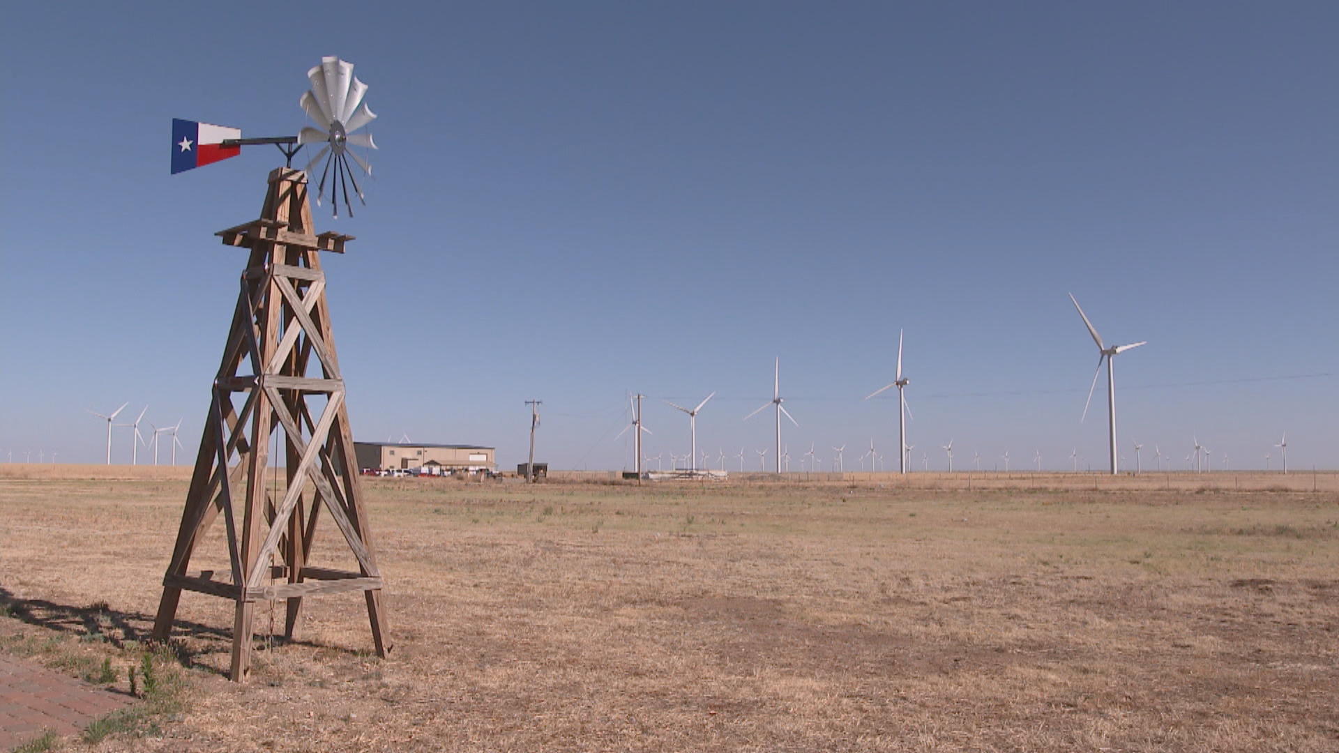
Figure 1. A Wind Farm in TX. With fast growing industry, wind electricity in Texas is slowly outpacing coal. (Source: CBS News, 2018)
0. Prepare the data.
#Filtering TX plants

plant_df_raw <- read_excel("egrid2018_data.xlsx", skip = 1, sheet = "PLNT18")

plant_tx_df <- plant_df_raw %>%
  filter(PSTATABB == "TX") %>%
  clean_names() %>%
  filter(plngenan >= 10000) %>%
  select(pstatabb, plprmfl, plfuelct, plngenan, lat, lon) %>%
  drop_na() %>%
  mutate(type = case_when(
    plfuelct %in% c("OFSL", "OTHF") ~ "OTHER",
    TRUE  ~ plfuelct
  )) %>%
  mutate(type = factor(type, levels = c("COAL", "OIL", "GAS", "BIOMASS", "NUCLEAR", "HYDRO", "WIND", "OTHER", "SOLAR"))) #Changing levels to make the color match the type later

plant_tx_sf <- st_as_sf(plant_tx_df, coords = c("lon", "lat"), crs = 4326)
raw1 <- read_excel("generation_monthly.xlsx", sheet = "2001_2002_FINAL")
raw2 <- read_excel("generation_monthly.xlsx", sheet = "2003_2004_FINAL")
raw3 <- read_excel("generation_monthly.xlsx", sheet = "2005-2007_FINAL")
raw4 <- read_excel("generation_monthly.xlsx", sheet = "2008-2009_FINAL")
raw5 <- read_excel("generation_monthly.xlsx", sheet = "2012_FINAL")
raw6 <- read_excel("generation_monthly.xlsx", sheet = "2013_FINAL")
raw7 <- read_excel("generation_monthly.xlsx", sheet = "2014_Final")
raw8 <- read_excel("generation_monthly.xlsx", sheet = "2015_Final")
raw9 <- read_excel("generation_monthly.xlsx", sheet = "2016_Preliminary")
raw10 <- read_excel("generation_monthly.xlsx", sheet = "2017_Preliminary")
raw11 <- read_excel("generation_monthly.xlsx", sheet = "2018_Preliminary")
raw12 <- read_excel("generation_monthly.xlsx", sheet = "2019_Preliminary")
raw13 <- read_excel("generation_monthly.xlsx", sheet = "2010-2011_FINAL")raw_df <- bind_rows(raw1, raw2, raw3, raw4, raw5, raw6, raw7, raw8, raw9, raw10, raw11, raw12, raw13) %>%
clean_names()tx_ts <- raw_df %>%
filter(state == "TX") %>%
filter(type_of_producer == "Total Electric Power Industry") %>%
filter(year != 2019) %>%
mutate(yearmonth = str_c(as.character(year), "/", as.character(month), "/", "1")) %>%
mutate(yearmonth = ymd(yearmonth)) %>%
mutate(ym_sep = yearmonth(yearmonth)) %>%
mutate(type = case_when(
energy_source == "Coal" ~ "COAL",
energy_source == "Petroleum" ~ "OIL",
energy_source %in% c("Natural Gas", "Other Gases" ) ~ "GAS",
energy_source == "Nuclear" ~ "NUCLEAR",
energy_source == "Hydroelectric Conventional" ~ "HYDRO",
energy_source == "Wind" ~ "WIND",
energy_source == "Solar Thermal and Photovoltaic" ~ "SOLAR",
energy_source %in% c("Wood and Wood Derived Fuels", "Other Biomass") ~ "BIOMASS",
energy_source == "Other" ~ "OTHER",
energy_source == "Total" ~ "TOTAL"
)) %>%
group_by(ym_sep, yearmonth, type) %>%
summarise(generation = sum(generation_megawatthours)) %>%
mutate(year = year(yearmonth),
month = month(yearmonth)) %>%
mutate(type = factor(type, levels = c("COAL", "OIL", "GAS", "BIOMASS", "NUCLEAR", "HYDRO", "WIND", "OTHER", "SOLAR", "TOTAL"))) #Changing levels to make the color match the type later
tx_ts_breakdown <- tx_ts %>%
filter(type != "TOTAL")
tx_ts_total <- tx_ts %>%
filter(type == "TOTAL")1. Geographic locations for TX power plants.
#Creating a TX map

us_county_raw <- read_sf(dsn = "cb_2018_us_county_500k", layer = "cb_2018_us_county_500k")

tx_map <- us_county_raw  %>%
  dplyr::filter(STATEFP == '48') %>%
  select(NAME) %>%
  st_transform(crs = 4326)

#plot(tx_map)
tx_plant_map <- ggplot(tx_map)+
geom_sf(fill = "white",
color = "black",
size = 0.2)+
geom_sf(data = plant_tx_sf,
aes(fill = type,
color = type,
size = plngenan/1000), #Unit in GWh
alpha = 0.8)+
scale_size(guide = "none") + #Removing size legend
labs(fill = "Plant Type",
color = "Plant Type")+
scale_fill_paletteer_d("ggsci::lanonc_lancet", direction = -1)+
scale_color_paletteer_d("ggsci::lanonc_lancet", direction = -1)
tx_plant_map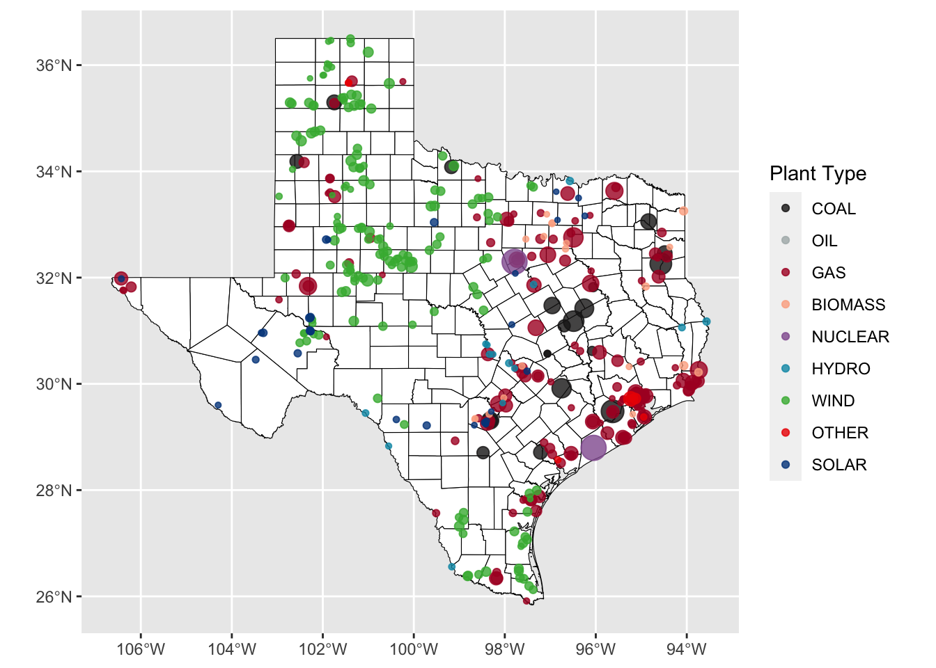
Figure 2. Geographic Locations of TX Power Plants. Each bubble on the map indicates a power plant. The color of the bubble indicates the type of the plant. The size of the bubble indicates the total generation amount of the plant in 2018. (Source: eGrid, 2018)
- Traditional large plants like coal, gas, and nuclear concentrate in the east region of the state.
- Small scale wind plants concentrates in the north and south region of the state.
2. TX generation mix change from 2001 to 2018.
tx_tsibble <- as_tsibble(tx_ts_breakdown, key = type, index = ym_sep) %>%
  fill_gaps()

tx_tsibble1 <- tx_tsibble %>%
  rename('Generation Type' = type) #Just changing the label name

tx_tsibble1 %>%
  autoplot(generation/1000)+
  scale_color_paletteer_d("ggsci::lanonc_lancet", direction = -1) +
  theme_classic()+
  scale_y_continuous(labels = scientific)+
  labs(y = "Generation (GWh)", x = "Year")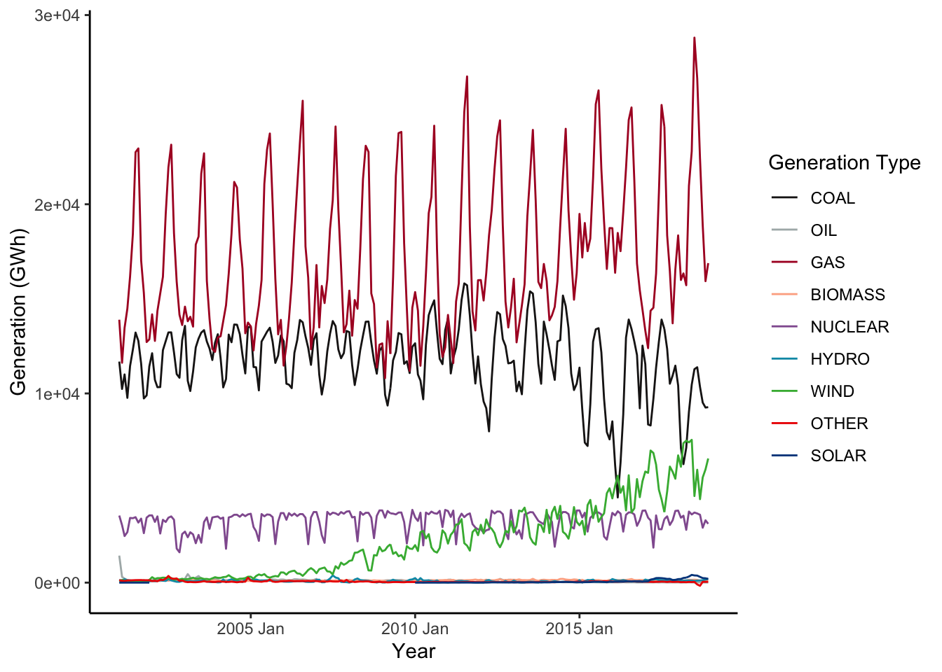
Figure 3. TX Generation Change from 2001 to 2018 by Generation Type. The color of the line indicates the generation type. Gas, coal, wind, and nuclear contributes the most to TX electricity. (Source: US EIA, 2020)
- Gas, coal and nuclear show strong seasonality.
- The seasonality for wind is less obvious.
- Coal shows a trend of decreasing.
- Wind shows a trend of increasing.
total_annually <- tx_ts_total %>%
  group_by(year) %>%
  summarise(generation = sum(generation))

total_annually_breakdown <- tx_ts_breakdown %>%
  group_by(year, type) %>%
  summarise(generation = sum(generation))


ggplot()+
  geom_line(data = total_annually,
            aes(x = year, y = generation/1000),
            size = 2)+
  scale_x_continuous(breaks=seq(2001,2018,1))+
  geom_bar(data = total_annually_breakdown,
           aes(x = year, y = generation/1000, fill = type),
           stat = "identity",
           width = 0.4,
           alpha = 0.8)+
  scale_fill_paletteer_d("ggsci::lanonc_lancet", direction = -1) +
  theme_classic()+
  labs(y = "Generation (GWh)", x = "Year", fill = "Generation Type") +
  scale_y_continuous(expand = c(0, 0))+
  theme(axis.text.x = element_text(angle = 45, hjust = 1))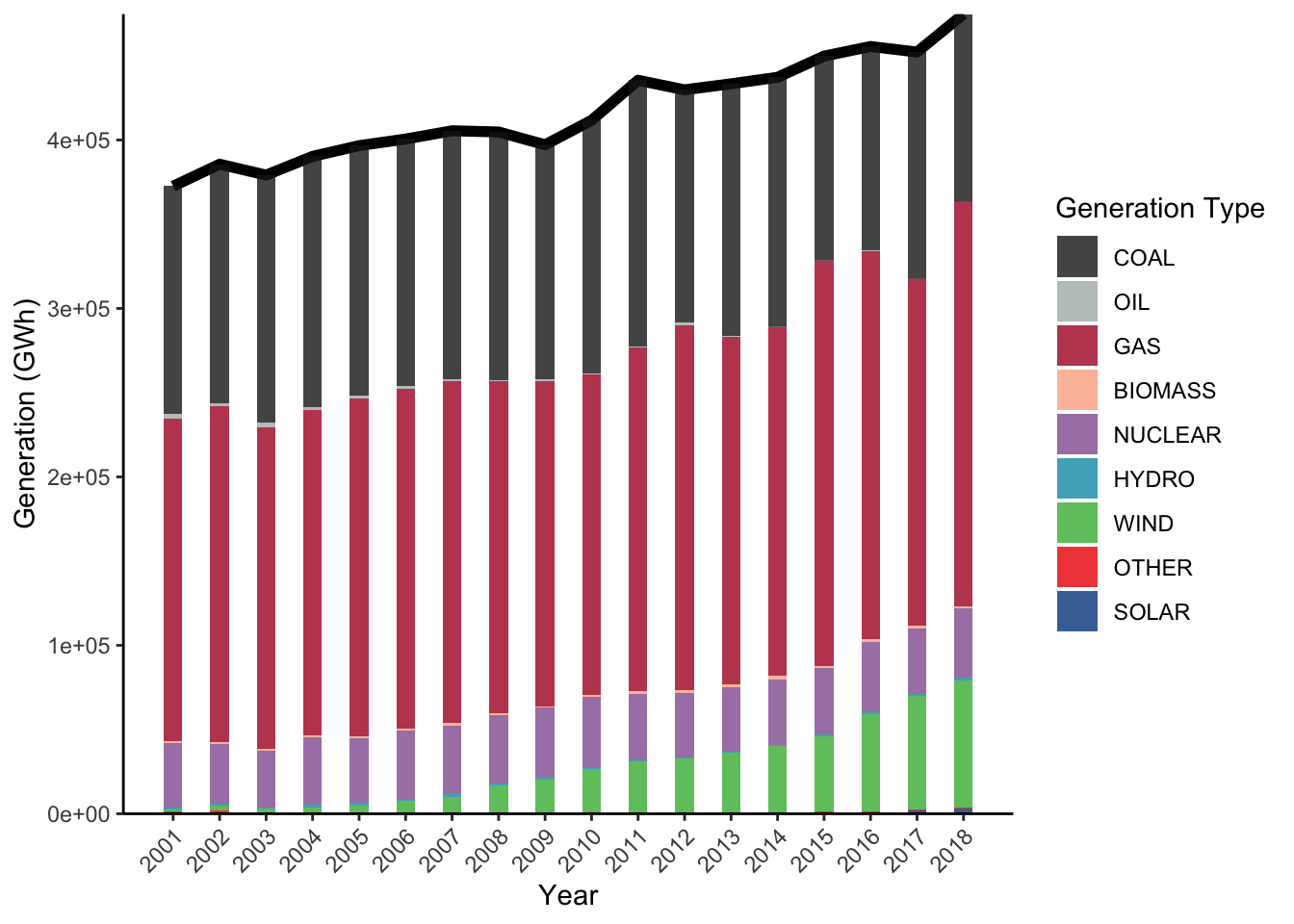
Figure 4. TX Generation Change from 2001 to 2018 in Total and in Breakdown. The black bold line indicates the total generation amount between 2001 to 2018. The color of the bar for each year indicates the mix of generation type.(Source: US EIA, 2020)
- In total, the electricity generation in TX shows an increasing trend.
3. The seasonal change of the generation amount for four main generation types.
tx_tsibble_major <- tx_tsibble %>%
  filter(type %in% c("GAS", "COAL", "NUCLEAR", "WIND"))

#tx_tsibble_major %>%
#  gg_season(generation, max_col = 100)+
#  scale_color_gradientn(colors = paletteer_d("ggsci::default_gsea"))

ggplot(data = tx_tsibble_major, aes(x = month, y = generation/1000, group = year))+
  geom_line(aes(color = year))+
  facet_wrap(~type,
             ncol = 1,
             scale = "free",
             strip.position = "right")+
  scale_color_gradientn(colors = paletteer_d("ggsci::default_gsea")) + #manually manipulating color
  theme_classic()+
  scale_y_continuous(labels = scientific)+
  scale_x_continuous(breaks=seq(1,12,1))+
  labs(y = "Generation (GWh)", x = "Month", color = "Year")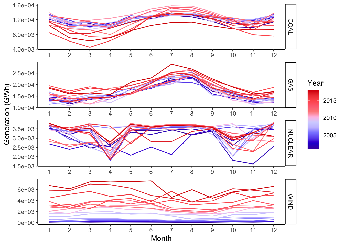
Figure 5. Season Plots for Coal, Gas, Nuclear, and Wind Generation in TX. A season plot shows the change of the generation in one year. Each line in the plot represents one year, indicated by the color scale. (Source: US EIA, 2020)
- For coal and gas, the generation pattern in one year follows the common pattern of high electricity demand in summer. As a result, the generation increases significantly during summer months to guarantee supply.
- However, nuclear and wind do not show such pattern, probably due to their continous generation characteristics and dependence on weather. In fact, the lack of flexibility is usually considered as a disadvantage of renewable powers.
- There are two significant generation drops for nuclear in October and April. This is probably due to the annual shutdown of the reactors.
- Similarly, the season plot indicates the decreasing of coal generation and the increasing of wind generation.
Reference:
- CBS News. (2018). A red state goes green: How Texas became a pioneer in wind energy. Available at: https://www.cbsnews.com/news/texas-leader-in-renewable-energy-wind-turbines/
- US EPA. (2020). Emissions & Generation Resource Integrated Database (eGRID). Available at: https://www.epa.gov/energy/emissions-generation-resource-integrated-database-egrid
- US EIA. (2020). Detailed preliminary EIA-923 monthly and annual survey data (back to 1990). Available at: https://www.eia.gov/electricity/data.php#generation
Yingfei "Ted" Jiang
Sustainability Specialist
客亦知夫水與月乎?逝者如斯,而未嘗往也;盈虛者如彼,而卒莫消長也。蓋將自其變者而觀之,則天地曾不能以一瞬;自其不變者而觀之,則物與我皆無盡也,而又何羨乎? 且夫天地之間,物各有主,茍非吾之所有,雖一毫而莫取。惟江上之清風,與山間之明月,耳得之而為聲,目遇之而成色,取之無禁,用之不竭,是造物者之無盡藏也,而吾與子之所共食。 –蘇軾《赤壁賦》
Do you happen to know the nature of water or the moon? Water is always on the run like this, but never lost in its course; the moon always waxes and wanes like that, but never out of its sphere. When viewed from a changing perspective, the universe can hardly be the same even within a blink of an eye, But when looked at from an unchanging perspective, everything conserves itself, and so do we. Therefore, what’s in them to be admired? Besides, in this universe, everything has its rightful owner. If something does not belong to you, then you shall not even have a bit of it. Only the refreshing breeze on the river and the bright moon over the hills are an exception. If you can hear it, it is a sound to you; if you can see it, it is a view to you. It never ends and is never exhausted. It is the infinite treasure granted to us by our Creator for both of us to enjoy. – Su Shi, Ode to the Red Cliff