US Coal Plants and Respiratory Conditions

Coal power plants are notorious for their \(NO_x\), \(SO_2\), and particulate matter emissions, which could all cause respiratory conditions. This project will map the large scale coal power plants (annual generation > 1000GWh) in the US, and the prevalance of three major respiratory conditions–chronic obstructive pulmonary disease (COPD), asthma, and lung and bronchus cancer– in all US states. Remember that this project will not do any regressions on the causality between coal power plants and respiratory conditions. Respiratory conditions are related to many factors such as mobile emissions, climate, geographic features, etc. Hence, it is irresponsible to use this project to make any declrations.

Figure 1. A Coal Power Plant in Kentucky. (Source: Luke Sharrett for The New York Times, 2016)

#Create separate CRS for AK, HI, and lower states

crs_lower48 <- "+proj=aea +lat_1=29.5 +lat_2=45.5 +lat_0=37.5 +lon_0=-96 +x_0=0 +y_0=0 +ellps=GRS80 +datum=NAD83 +units=m +no_defs"
crs_ak <- "+proj=aea +lat_1=55 +lat_2=65 +lat_0=50 +lon_0=-154 +x_0=0 +y_0=0 +ellps=GRS80 +towgs84=0,0,0,0,0,0,0 +units=m +no_defs "
crs_hi <- "+proj=aea +lat_1=8 +lat_2=18 +lat_0=13 +lon_0=-157 +x_0=0 +y_0=0 +ellps=GRS80 +datum=NAD83 +units=m +no_defs"

plant_df_raw <- read_excel("egrid2018_data.xlsx", skip = 1, sheet = "PLNT18")

plant_df <- plant_df_raw %>% 
  filter(! PSTATABB %in% c("PR", "AS", "VI", "GU", "MP")) %>% 
  clean_names() %>% 
  select(pstatabb, plprmfl, plfuelct, plngenan, lat, lon) %>% 
  drop_na() %>% 
  filter(plfuelct != "OTHF") %>% 
  filter(plngenan > 1000000) %>% 
  mutate(renewable = case_when(
    plfuelct %in% c("WIND", "HYDRO", "BIOMASS", "SOLAR", "NUCLEAR", "GEOTHERMAL") ~ "Renewable",
    TRUE  ~ str_to_title(plfuelct)
  ))

plant_sf <- st_as_sf(plant_df, coords = c("lon", "lat"), crs = 4326)

plant_coal_sf <- plant_sf %>% 
  filter(plfuelct == "COAL")

us_map_raw <- read_sf(dsn = "cb_2018_us_state_500k", layer = "cb_2018_us_state_500k")
  
us_map <- us_map_raw %>%   
  filter(! STUSPS %in% c("PR", "AS", "VI", "GU", "MP")) %>% 
  select(STUSPS) %>% 
  st_transform(crs = 4326)

#plot(us_map)

med_raw <- read_csv("U.S._Chronic_Disease_Indicators__CDI_.csv")

#Including data on copd, lung cancer, and asthma in the data frame

#Adding COPD
med_copd <- med_raw %>% 
  filter(Topic == "Chronic Obstructive Pulmonary Disease") %>% 
  filter(DataValueType == "Age-adjusted Prevalence") %>% 
  filter(YearStart == 2018) %>% 
  filter(Stratification1 == "Overall") %>% 
  filter(LocationAbbr != "US") %>% 
  filter(Question == "Prevalence of chronic obstructive pulmonary disease among adults >= 18") %>% 
  filter(! LocationAbbr %in% c("PR", "AS", "VI", "GU", "MP")) %>% 
  mutate(STUSPS = LocationAbbr) %>% 
  select (STUSPS,
          copd = DataValue)

med_sf <- left_join(us_map, med_copd)

#Adding asthma
med_asthma <- med_raw %>% 
  filter(Topic == "Asthma") %>% 
  filter(DataValueType == "Age-adjusted Prevalence") %>% 
  filter(YearStart == 2018) %>% 
  filter(Stratification1 == "Overall") %>% 
  filter(LocationAbbr != "US") %>% 
  filter(Question == "Current asthma prevalence among adults aged >= 18 years") %>% 
  filter(! LocationAbbr %in% c("PR", "AS", "VI", "GU", "MP")) %>% 
  mutate(STUSPS = LocationAbbr) %>% 
  select (STUSPS,
          asthma = DataValue)

med_sf <- left_join(med_sf, med_asthma) 

#Adding cancer
med_cancer <- med_raw %>% 
  filter(Topic == "Cancer") %>% 
  filter(Question == "Cancer of the lung and bronchus, incidence") %>% 
  filter(DataValueType == "Average Annual Age-adjusted Rate") %>% 
  filter(YearStart == 2012) %>% 
  filter(Stratification1 == "Overall") %>% 
  filter(LocationAbbr != "US") %>% 
  filter(! LocationAbbr %in% c("PR", "AS", "VI", "GU", "MP")) %>% 
  mutate(STUSPS = LocationAbbr) %>% 
  select (STUSPS,
          cancer = DataValue)

med_sf <- left_join(med_sf, med_cancer)

#Trying to move AK and HI

med_main <- med_sf %>% 
  filter(!STUSPS %in% c("AK", "HI")) %>% 
  st_transform(crs_lower48)

bb <- st_bbox(med_main)

med_ak <- med_sf %>% 
  filter(STUSPS == "AK") %>% 
  st_transform(crs_ak)

med_hi <- med_sf %>% 
  filter(STUSPS == "HI") %>% 
  st_transform(crs_hi)

#Same thing for power plants

coal_main <- plant_coal_sf %>% 
  filter(! pstatabb %in% c("AK", "HI")) %>% 
  st_transform(crs_lower48)

coal_ak <- plant_coal_sf %>% 
  filter(pstatabb == "AK") %>% 
  st_transform(crs_ak)

coal_hi <- plant_coal_sf %>% 
  filter(pstatabb == "HI") %>% 
  st_transform(crs_hi)

#Trying to plot (and hope it works).
copd_main <- ggplot(med_main) +
  geom_sf(color = "black", 
          aes(fill = copd),
          size = 0.2) +
  scale_fill_gradientn(colors = paletteer_d("dichromat::BluetoOrange.12"),
                       limits = c(3, 14)) +
  labs(fill = "Percent (%)") +
  geom_sf(data = coal_main,
          color = "black",
          alpha = 0.8,
          show.legend = FALSE
          )+
  ggtitle("Large Scale Coal Power Plants and Prevalence of\nCOPD among adults >= 18 in United States")

copd_ak <- ggplot(med_ak) +
  geom_sf(color = "black", 
          aes(fill = copd),
          size = 0.2,
          show.legend = FALSE) +
  scale_fill_gradientn(colors = paletteer_d("dichromat::BluetoOrange.12"),
                       limits = c(3, 14)) +
  labs(fill = "Percent (%)") +
  geom_sf(data = coal_ak,
          color = "black",
          alpha = 0.8,
          show.legend = FALSE
          )

copd_hi <- ggplot(med_hi) +
  geom_sf(color = "black", 
          aes(fill = copd),
          size = 0.2,
          show.legend = FALSE) +
  scale_fill_gradientn(colors = paletteer_d("dichromat::BluetoOrange.12"),
                       limits = c(3, 14)) +
  labs(fill = "Percent (%)") +
  geom_sf(data = coal_hi,
          color = "black",
          alpha = 0.8,
          show.legend = FALSE
          )

#Pasting HI an AK to the lower states

ggarrange(
  copd_main,
  ggarrange(copd_ak, copd_hi),
  nrow = 2,
  heights = c(1, 0.5)
)

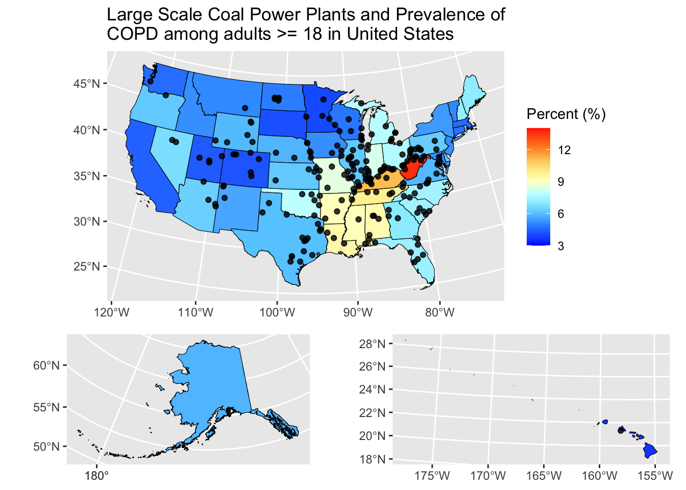
Figure 2. Large Scale Coal Power Plants and Prevalence of COPD among Adults >= 18 in United States. Each point on the map represents a large scale coal power plant. The color of the state indicates the prevalence of COPD among adults >= 18. (Source: eGrid, 2018. US CDC, 2020.)

asthma_main <- ggplot(med_main) +
  geom_sf(color = "black", 
          aes(fill = asthma),
          size = 0.2) +
  scale_fill_gradientn(colors = paletteer_d("dichromat::BluetoOrange.12"),
                       limits = c(7, 13)) +
  labs(fill = "Percent (%)") +
  geom_sf(data = coal_main,
          color = "black",
          alpha = 0.8,
          show.legend = FALSE
          )+
  ggtitle("Large Scale Coal Power Plants and Prevalence of\nAsthma among adults >= 18 in United States")

asthma_ak <- ggplot(med_ak) +
  geom_sf(color = "black", 
          aes(fill = asthma),
          size = 0.2,
          show.legend = FALSE) +
  scale_fill_gradientn(colors = paletteer_d("dichromat::BluetoOrange.12"),
                       limits = c(7, 13)) +
  labs(fill = "Percent (%)") +
  geom_sf(data = coal_ak,
          color = "black",
          alpha = 0.8,
          show.legend = FALSE
          )

asthma_hi <- ggplot(med_hi) +
  geom_sf(color = "black", 
          aes(fill = asthma),
          size = 0.2,
          show.legend = FALSE) +
  scale_fill_gradientn(colors = paletteer_d("dichromat::BluetoOrange.12"),
                       limits = c(7, 13)) +
  labs(fill = "Percent (%)") +
  geom_sf(data = coal_hi,
          color = "black",
          alpha = 0.8,
          show.legend = FALSE
          )

ggarrange(
  asthma_main,
  ggarrange(asthma_ak, asthma_hi),
  nrow = 2,
  heights = c(1, 0.5)
)

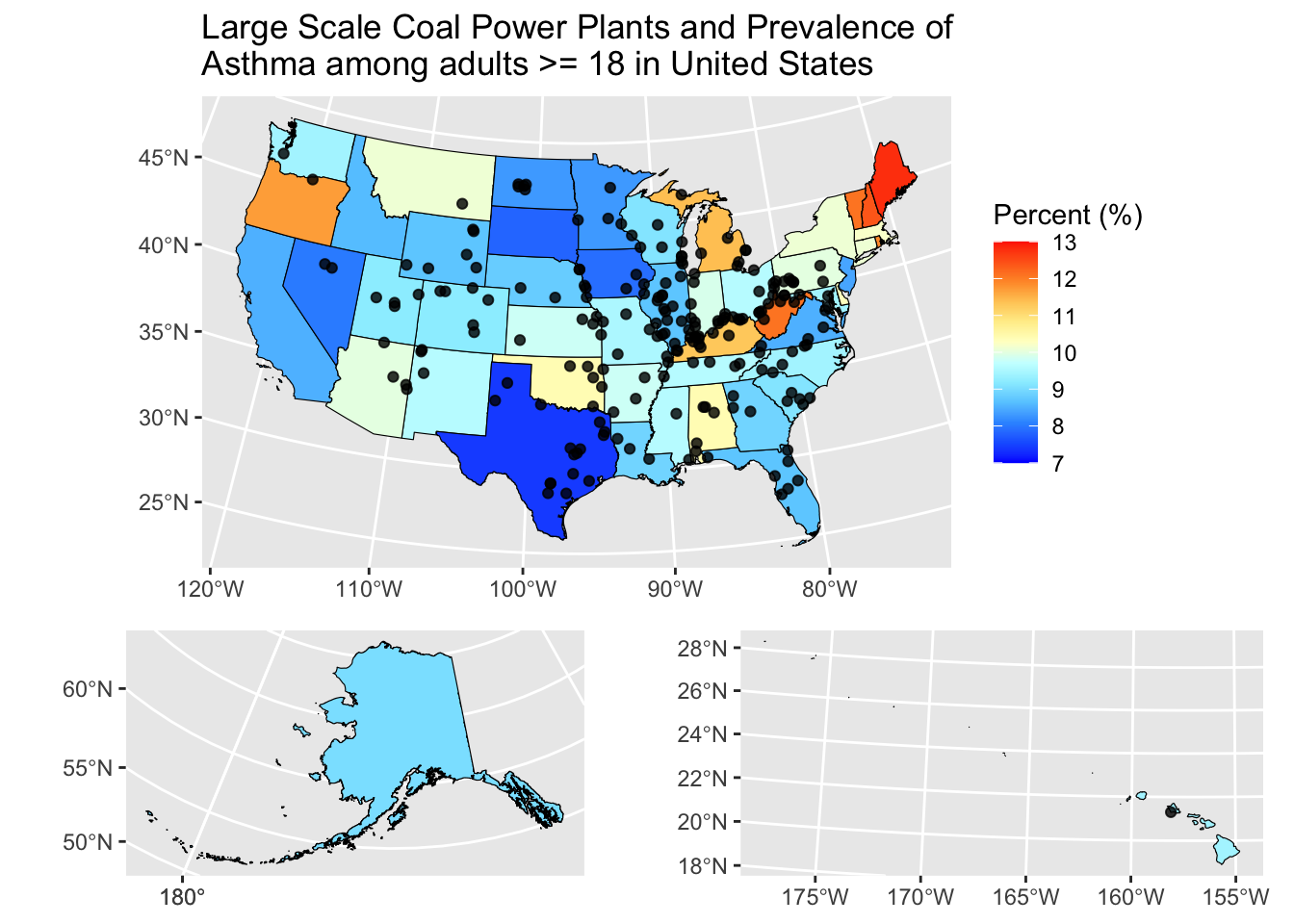
Figure 3. Large Scale Coal Power Plants and Prevalence of Asthma among Adults >= 18 in United States. Each point on the map represents a large scale coal power plant. The color of the state indicates the prevalence of asthma among adults >= 18. (Source: eGrid, 2018. US CDC, 2020.)

cancer_main <- ggplot(med_main) +
  geom_sf(color = "black", 
          aes(fill = cancer),
          size = 0.2) +
  scale_fill_gradientn(colors = paletteer_d("dichromat::BluetoOrange.12"),
                       limits = c(25, 95)) +
  labs(fill = "Percent (%)") +
  geom_sf(data = coal_main,
          color = "black",
          alpha = 0.8,
          show.legend = FALSE
          )+
  ggtitle("Large Scale Coal Power Plants and Incidence of\nLung and Bronchus Cancer in United States")

cancer_ak <- ggplot(med_ak) +
  geom_sf(color = "black", 
          aes(fill = cancer),
          size = 0.2,
          show.legend = FALSE) +
  scale_fill_gradientn(colors = paletteer_d("dichromat::BluetoOrange.12"),
                       limits = c(25, 95)) +
  labs(fill = "Percent (%)") +
  geom_sf(data = coal_ak,
          color = "black",
          alpha = 0.8,
          show.legend = FALSE
          )

cancer_hi <- ggplot(med_hi) +
  geom_sf(color = "black", 
          aes(fill = cancer),
          size = 0.2,
          show.legend = FALSE) +
  scale_fill_gradientn(colors = paletteer_d("dichromat::BluetoOrange.12"),
                       limits = c(25, 95)) +
  labs(fill = "Percent (%)") +
  geom_sf(data = coal_hi,
          color = "black",
          alpha = 0.8,
          show.legend = FALSE
          )

ggarrange(
  cancer_main,
  ggarrange(cancer_ak, cancer_hi),
  nrow = 2,
  heights = c(1, 0.5)
)

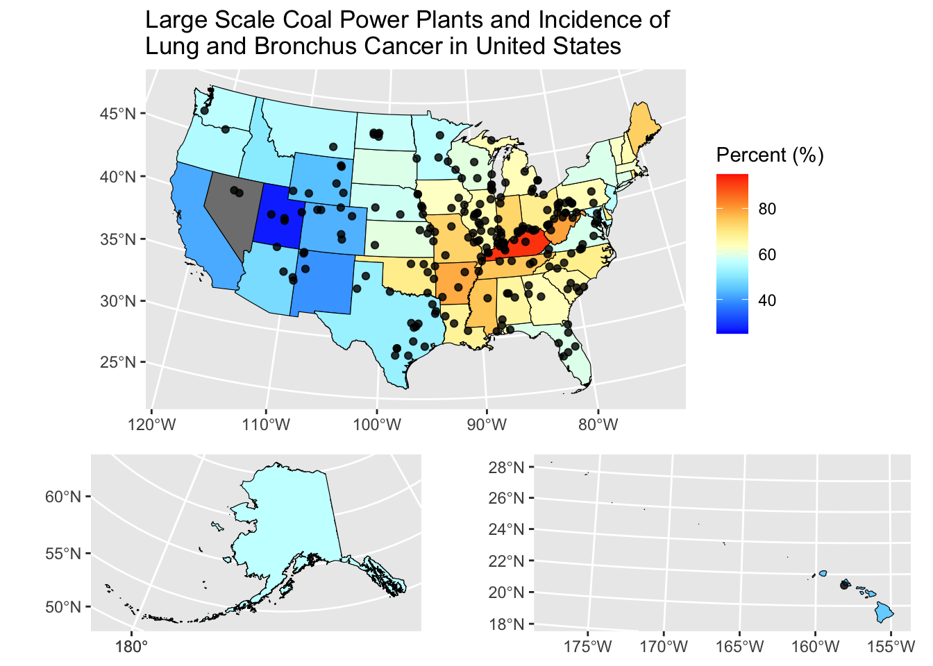
Figure 4. Large Scale Coal Power Plants and Incidence of Lung and Bronchus Cancer in United States. Each point on the map represents a large scale coal power plant. The color of the state indicates the prevalence of incidence of lung and bronchus cancer. The cancer data for NV is not statistically significant thus the missing value. (Source: eGrid, 2018. US CDC, 2020.)